Generating Baby Names - Intro to Encoders, Decoders, and Fine-Tuning

Part 1 - Encoders

With the current hype of generative AI, I see a lot of people jumping into it without understanding what it is. As much as I’d love to just immediately make a post on generative AI, I want to focus more on applications in AI through examples. You may ask, “why not just use ChatGPT to generate a list of baby names?”. But what if instead of generating baby names I wanted to extract all proper nouns, verbs, and adverbs from a sentence? Again, you might ask “why not just use ChatGPT to do this?”. These are two different tasks — one focussed on an encoder and one focussed on a decoder. While ChatGPT may be able to solve these, it’s a potentially expensive (in multiple ways) solution. Instead, in this 3 part post, we’ll look at how we can use machine learning to learn names and generate potentially novel ones. Along the way you’ll see what we gain from an encoder, how to perform transfer learning, and several ways to decode (generate). This post will be focussed on training the encoder, so let’s get started. If you want to download the notebook, you can find it on my GitHub.

Encoders

First let’s start with what an encoder is. If you’re familiar with Natural Language Processing (NLP) you may already know. If you’ve heard of BERT, you might think an encoder is a transformer. But really, the transformer architecture is just that — an architecture. An encoder can be thought of as a learned way to represent input as a vector. Let’s take names as an example. How do you represent “Chris” to a computer? Ultimately the computer needs numbers to work with. We could just decide to generate a random vector and assign it to a name, but this will mean there’s no connection between the vector and the actual name. This is why these representations are learned. The way they’re learned can vary, but in this post we’ll be looking at next character prediction.

Here we’ll be placing a 128 dimension vector right before the next character prediction. As the model trains and learns how to correctly generate a character given a partial sequence, it will also learn how to assign weights to the vector in order to make classification better. That 128 dimension vector is the learned encoding! Once the training is complete, that vector can be used for a number of things including transfer learning, fine-tuning, and decoding.

Gathering Data

The first thing we’ll need is some data. I’ll be using a list of baby names I found here. This is easy enough using pandas:

url = 'https://raw.githubusercontent.com/hadley/data-baby-names/master/baby-names.csv'
content = requests.get(url).content
df = pd.read_csv(io.StringIO(content.decode('utf-8')))
df.head()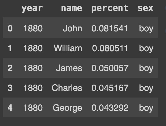

Great! So it has names by year, the percentage of babies with that name, and the sex of the child with that name. Right off the bat it should be noted that this list is not all inclusive. In fact, scrolling through you’ll see very common names, but there is appears to be a cutoff of popularity where the names are no longer included.

Next we’ll drop duplicates. We don’t need “Alex” showing up twice if it’s included for both boy and girl names.

df_unique = df['name'].drop_duplicates().reset_index(drop=True)
len(df_unique) # 6782

Next we’ll split the names into a training, validation, and test set. This is a normal process in supervised learning approaches, but first let’s discuss why we’re doing this here. During training the goal will be to have a model learn what character comes next based on the characters it’s seen. This is a probability distribution over 26 classes in this case — one for each letter in the English alphabet. I’m specifically using the validation set to determine at what point we begin overfitting the training set, and will be using that as a stopping point. So why have a test set? Well, in the post covering fine-tuning I’ll use the test set. So for now I want to leave some names out on purpose.

Here is a common way to split a pandas DataFrame into train, val, and test:

train_percent = .8
val_percent = .1
test_percent = .1

df_train = df_unique.sample(frac=train_percent, random_state=0xC0FFEE)
df_val_test = df_unique.drop(df_train.index).sample(frac=1.0, random_state=0xC0FFEE)
df_val = df_val_test.sample(frac=0.5, random_state=0xC0FFEE)
df_test = df_val_test.drop(df_val.index)

Great! Now we have data for different parts of our pipeline. Next we’ll look at how to preprocess the data.

Preprocessing Data

Right now we have a bunch of names, or strings. A common pipeline for preprocessing might include lowercasing words, splitting hyphenated words into two, separating punctuation, etc. Here we’re only concerned with some simple tokenization. Tokenization is essentially splitting words into a smaller representation called tokens. We’ll explore this in more detail in future posts, but right now we just need a way for the machine learning algorithm to know when it’s looking at a name. To do this we’ll split words into simple character tokens and include three special tokens: <sos>, <eos>, and <pad>. The <sos> token stands for start-of-sequence, and will be used to denote the beginning of a name. Similarly, <eos> is end-of-sequence and will denote the end of a name. We also have <pad> which is a padding token.

Let’s start by creating a mapping from a token to an index. This index will be the index into the vocabulary which can be fed into an Embedding layer, or one-hot encoding layer, representing the word.

chars = ['<pad>'] + ['<sos>'] + list(string.ascii_lowercase) + ['<eos>']
char_to_idx = {char:idx for idx,char in enumerate(chars)}
idx_to_char = {idx: char for char,idx in char_to_idx.items()}
vocab_size = len(char_to_idx)
print(vocab_size)  # 29

I’m explicitly putting the <pad> token first so that it maps to 0. I’ll explain this in detail later in this post, but for now, just keep a mental note of that. Also note that the vocabulary size is 29 as this comes up again in the model architecture.

Now we can create a helper function to take a name and return a tokenized name:

def get_tokenized_names(df):
  names = df.values
  ret = []
  for name in names:
    name = name.lower()
    toks = ['<sos>'] + list(name) + ['<eos>']
    ret.append(toks)
  return ret

>>> get_tokenized_names(df_val)[:5]
[['<sos>', 'o', 'r', 'i', 'o', 'n', '<eos>'],
 ['<sos>', 'l', 'i', 'b', 'b', 'y', '<eos>'],
 ['<sos>', 'n', 'o', 'l', 'a', '<eos>'],
 ['<sos>', 'r', 'o', 's', 'i', 'e', '<eos>'],
 ['<sos>', 'r', 'e', 'y', '<eos>']]

Next we need a way to sample this data. For this we’'ll use PyTorch’s Dataset class:

class NameDataset(Dataset):
  def __init__(self, tokenized_names, char_to_id):
    self.tok_names = tokenized_names
    self.char_to_id = char_to_id

    self._samples = []
    for tok_name in self.tok_names:
      for i in range(len(tok_name) - 1):
        partial_seq = [self.char_to_id[tok] for tok in tok_name[:i + 1]]
        next_tok = self.char_to_id[tok_name[i+1]]
        self._samples.append((partial_seq, next_tok))

  def __len__(self):
    return len(self._samples)

  def __getitem__(self, idx):
    return self._samples[idx]

This might seem a bit confusing, but all this does is build a list of samples consisting of a tuple of (partial sequence, next token). Then, when we sample from the dataset, we can get some partial sequence of tokens followed by the token that’s expected. For instance, if you only have the name “Orion”, your list of samples would look like this:

[([1], 16),
 ([1, 16], 19),
 ([1, 16, 19], 10),
 ([1, 16, 19, 10], 16),
 ([1, 16, 19, 10, 16], 15),
 ([1, 16, 19, 10, 16, 15], 28)]

Above are the numerical indices for the tokens, which correspond to the following:

<sos> -> o
<sos> o -> r
<sos> o r -> i
<sos> o r i -> o
<sos> o r i o -> n
<sos> o r i o n -> <eos>

Awesome! Now we can sample some partial sequence and try to predict the next character! Next let’s build the language model.

Language Model (and some math)

Oh cool! LLMs! Just kidding. This is going to be a small language model. Normally these are just referred to as LMs or simply language models. The language model will be a bidirectional LSTM with a final layer of 29 nodes. If you recall, the vocabulary for our data has 29 tokens, which is why we have 29 nodes. I won’t post the entire code here, but you can check it out on my GitHub. Instead, I want to focus on the more interesting forward() method:

def forward(self, seqs):
    # Count the non-pad tokens (part 1)
    seq_lens = torch.count_nonzero(seqs, dim=1).cpu()
    embeddings = self.embedding(seqs)

    # Feed through LSTM (part 2)
    _, (hn, _) = self.lstm(
        nn.utils.rnn.pack_padded_sequence(
            embeddings,
            seq_lens,
            batch_first=True,
            enforce_sorted=False
        )
    )
    # Save off hidden state before FC (part 3)
    self.hidden = torch.cat((hn[0], hn[1]), dim=1)
    out = self.fc(self.hidden)
    return out

Part 1

We’re just going to be counting the non-zero tokens. Remember, I specifically had the <pad> token be 0. By counting non-zero tokens, we’re looking at tokens that actually matter. Then we’ll feed the sequence of numbers into the embedding layer. This allows the model to learn a vector representation for the tokens. Maybe this means the model learns to put vowels near each other, or characters that have similar sounds such as C and K. We won’t be worrying about that here.

Part 2

Some “magic” happens. And if you don’t care, feel free to skip this explanation as it gets a bit mathy, but just know it helps speed up computations by quite a bit! Right now when we sample from the dataset, we’ll get a shape of (batch_size, n), however, n isn’t the same for each sample. Even if we just sampled three partial sequences from the “Orion” example above we could end up with this:

[([1], 16),
 ([1, 16], 19),
 ([1, 16, 19], 10)]

To avoid this we’ll be using a collate function to pad the sequences to be the same length. This would result in the following assuming the above was a batch (ignoring the next token for now):

[[1, 0, 0]
 [1, 16, 0]
 [1, 16, 19]]

Now for simplicity let’s say we have a column vector [1, 2, 3]. Let’s call this vector b, and the matrix of partial sequences A. If we do A.T @ b we get the following:

>>> A.T @ b
array([[ 6],
       [80],
       [57]])

But there’s actually quite a bit of unnecessary work going on there. Breaking this down we get:

[[1*1 + 2*1  + 3*1],
 [1*0 + 2*16 + 3*16],
 [1*0 + 2*0  + 3*19]]

So literally 3/9 or 33% of our multiplications are with 0. A better way to do this is instead to use pack_padded_sequence() like so:

>>> ps = pack_padded_sequence(A.T, lengths=[1,2,3], enforce_sorted=False)
>>> ps
PackedSequence(data=tensor([ 1,  1,  1, 16, 16, 19]), batch_sizes=tensor([3, 2, 1]), sorted_indices=tensor([2, 1, 0]), unsorted_indices=tensor([2, 1, 0]))
>>> batch_idxs = torch.cumsum(torch.cat((torch.tensor([0]), ps.batch_sizes), dim=-1),0)
>>> batch_idxs
tensor([0, 3, 5, 6])

Now because it’s essentially unrolled, we can look at the individual slices we get from the batch_idxs from [0:3], [3:5] and [6] and end up with this:

A: tensor([1, 1, 1]) @ b tensor([3, 2, 1]) = 6
A: tensor([16, 16]) @ b tensor([3, 2]) = 80
A: tensor([19]) @ b tensor([3]) = 57

Bam! No more multiplication with 0. Might not seem like a big deal here, but if you can save time during ML training…. you’ll be very happy.

Part 3

Just need to concatenate the final state of the bidirectional LSTM and feed it through the fully connected layer. Because it’s bidirectional you have a vector from left→right and a vector from right→left. In this case we can simply stack them. You might notice that the self.fc part is dealing with the multi-class classification. If you remember from the beginning of the post I mentioned the vector right before that is our encoding. This means that self.hidden will hold the 128 dimension vector representing the encoding.

Collate

Next we’ll define a collate() function. This function will handle the batch before it gets fed to the model. All it needs to do is pad the sequence so we don’t have a jagged matrix. Below is the code:

def collate(batch):
  partials, next_toks = [], []
  for (partial, next_tok) in batch:
    partials.append(torch.tensor(partial))
    next_toks.append(next_tok)

  return (
      pad_sequence(partials, batch_first=True, padding_value=0),
      torch.tensor(next_toks)
  )

Here I explicitly state the padding_value to be 0. You can make the padding value something besides one, but remember that by treating it as zero you can gain some additional benefits listed in Part 2 above.

Now if you took a batch size of 3 from a data loader, you could end up with this:

>>> next(iter(DataLoader(val_ds, batch_size=3, collate_fn=collate, shuffle=True)))

(tensor([[ 1, 14,  6, 19, 19],
         [ 1,  9,  0,  0,  0],
         [ 1,  6, 13, 16,  0]]),
 tensor([10,  2, 26]))

Now that we have the language model defined we need to train it!

Training

We have the model defined and now we just need to train it. To do this it’s just multi-class classification. We take a batch of partial sequences, try to predict the next token, apply cross-entropy loss, and bam! Language model! We can start by getting a training and validation DataLoader:

train_dataloader = DataLoader(
     NameDataset(get_tokenized_names(df_train), char_to_idx),
     batch_size=256,
     collate_fn=collate,
     shuffle=True
)

val_dataloader = DataLoader(
     NameDataset(get_tokenized_names(df_val), char_to_idx),
     batch_size=256,
     collate_fn=collate,
     shuffle=True
)

This will allow us to sample from the NameDataset we created above and use the collate() function as well.

We can use PyTorch Lightning to allow for easier training. If you’ve never used it, it’s pretty handy. Rather than explicitly writing training and validation loops, you can instead inherit from a LightningModule and override some functions. Here is how we can do that:

class LitModel(pl.LightningModule):
  def __init__(self, encoder):
    super().__init__()
    self.encoder = encoder

  def _generic_step(self, batch, batch_idx):
    X, y = batch
    out = self.encoder(X)
    loss = F.cross_entropy(out, y)
    return loss

  def forward(self, seq):
    return self.encoder(seq)

  def training_step(self, batch, batch_idx):
    return self._generic_step(batch, batch_idx)

  def validation_step(self, batch, batch_idx):
    loss = self._generic_step(batch, batch_idx)
    self.log('val_loss', loss, prog_bar=True)
    return loss

  def configure_optimizers(self):
    opt = torch.optim.Adam(self.encoder.parameters(), lr=2e-3)
    return opt

Next we instantiate it and pass in the data loaders:

encoder = LM(vocab_size, 8, 64, 2)
lit_model = LitModel(encoder)

trainer = pl.Trainer(
    accelerator='auto',
    max_epochs=100,
    log_every_n_steps=25,
    callbacks=[
        RichProgressBar(refresh_rate=50),
        EarlyStopping(monitor='val_loss', mode='min', patience=3)
    ]
)

trainer.fit(lit_model, train_dataloader, val_dataloader)

This will set up a training loop and fit the model to the training data, while monitoring the validation loss. This will train the model for 100 epochs or until the validation loss has not improved for 3 epochs, whichever comes first.

And now you’ve trained a language model to do next character prediction for names! Now we can extract the 128 dimension vector.

Vector Representation

Now that the model is trained, we should also have a way to represent a name as a vector. However, if we simply pass a name to the model we’ll get a 29 dimension vector as the output. That’s because the model is still set up for doing multi-class classification. We could pass the name through the model, then manually extract the self.hidden layer, but that’s a lot of effort. Instead, a common approach is to replace the last fully connected layer with an Identity layer. This makes it so now when the model returns a vector, it’s actually the self.hidden layer! Below is how we can do that:

>>> enc = copy.deepcopy(lit_model.encoder).eval() 
>>> enc.fc = nn.Identity()
>>> enc

LM(
  (embedding): Embedding(29, 8)
  (lstm): LSTM(8, 64, num_layers=2, batch_first=True, bidirectional=True)
  (fc): Identity()
)

Now we can create a function to take a name and return the indices associated with the tokens. Once we do that, we can simply pass a name to the model and get a vector representation!

def name2token_ids(name):
  tok_name = ['<sos>'] + list(name.lower()) + ['<eos>']
  ids = [char_to_idx[tok] for tok in tok_name]
  return torch.tensor(ids).unsqueeze(0)

And now….

>>> enc(name2token_ids('chris')).shape

torch.Size([1, 128])

Conclusion

Congrats! You did it! In this post you created a dataset for next character prediction for names. You did a simple preprocessing technique and created the 29 token vocabulary. Afterwards you trained the model and performed early stopping. Then you swapped out the fully connected layer for an Identity layer, allowing us to produce the vector representation we were interested in. In the next post we’ll look at how to utilize that vector, and in the following we’ll use it to generate the names!